DOME files

Even very detailed datasets often lack complete data for crop model simulation. DOME (Data Overlay for Multi-model Export) files can be used to supply additional information to supplement data collected in a field experiment or farm survey. Use of a DOME does not alter the original dataset. Multiple DOMEs can be combined to create complex scenarios for simulation, making these a powerful tool for generating hypothetical scenarios from real data.

DOME functions have been developed to allow a modeler to estimate missing modeling inputs such as initial water content, initial N distribution, soil properties, and planting dates. Descriptions of these functions are listed here.

There are three kinds of DOME files:

Field overlay DOMEs add information to supplement a baseline simulation. These data are used in addition to data collected in the field and are provided solely to complete model input data required for this baseline simulation.
Seasonal Strategy DOMEs allow a single season of data to be used with multiple years of weather data to analyze scenarios based on seasonal weather variability. These DOMEs are used in conjunction with Field overlay DOMEs. Additional hypothetical management information may be introduced to mimic adaptations or other scenarios.
Batch DOMEs allow loops of simulations to be done for sensitivity analyses, climate change studies, and other simulation series.

The various parts of a DOME file are explained below. This is not an exhaustive explanation of all capabilities of DOMEs, but is meant to give the user a feel for the way DOME files are constructed and some of the capabilities.

As an example, we will look at the Field overlay DOME used for the Hot Serial Cereal experiment (Kimball et al., 2016). This is the same experiment described in the ‘AgMIP Translators’ description. The screenshots are equivalent to the data in the Field_overlay_HSC_v4.5a.csv file, but have been put into an Excel spreadsheet for a simpler view of data definitions. This Field overlay file can be downloaded here.

General notes on the DOME file structure:

Comments are denoted with ‘!’ and are not processed by the translators. Fields beginning with ‘!’ are ignored. Lines with ‘!’ in column 1 are entirely ignored.
Lines of data with ‘&’ in column 1 are processed by the translators.
The second column of every data line contains operators: INFO (for metadata), FILL (to fill in missing values), or REPLACE (to replace all values with the data provided).
The third column contains the name of the variable being estimated or set by the user.
The fourth column contains either a value or a function name.
All function names include “()” after the function name. Columns 5 through N after a function name contain function parameters.
Functions are applied in order, so if variable B depends on variable A, then variable A must be specified prior to variable B.
See more about DOME functions here

Metadata section

The metadata section at the top of every DOME file contains the full description of the scenario being modeled. This section is used by AgMIP Regional Integrated Assessment Teams to carry consistent metadata throughout workflows to provide provenance to final model outputs. Fields that are not relevant to a simulation may be left blank, but as a minimum, the DOME region identification (REG_ID) must be filled.

The DOME name is constructed from a concatenation of each metadata field (orange block above), separated by a dash. It is important to not use dashes in the field identifier text for this reason. The DOME name is used to link multiple DOMEs to the corresponding data elements.

Initial conditions

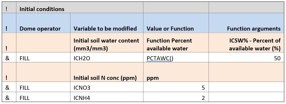
The initial conditions block is often needed in simulations if the soil water and nitrogen contents were not measured at the beginning of the simulation. Modelers must make their best evaluation of field conditions. Several DOME functions facilitate this process.

In this example, initial soil water content (ICH2O) was estimated using the PCTAWC function (percent available water). The user estimated that at the beginning of simulation that soil water content in each layer of the soil profile was 50% between lower limit and drained upper limit.

The initial soil nitrate (ICNO3) and ammonium (ICNH4) values are provided as values. These variables are arrays and so the same value is used for every element of the array. In this case, initial nitrate concentration is set to 5 ppm and ammonium to 2 ppm in every soil layer. The csv form of this initial conditions section would look like this:

Planting data.

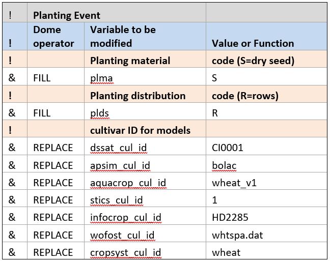
Planting and soil data are similarly filled with modeler-supplied parameters. Some of the values might be specific to a particular model. For example, in the Planting Event section, cultivar names specific to each model are provided. The model ID is used as a prefix for each. In this case, the “REPLACE” operator is used to provide cultivar names. These names will override any cultivar IDs in the data, if they are provided.

Soil data

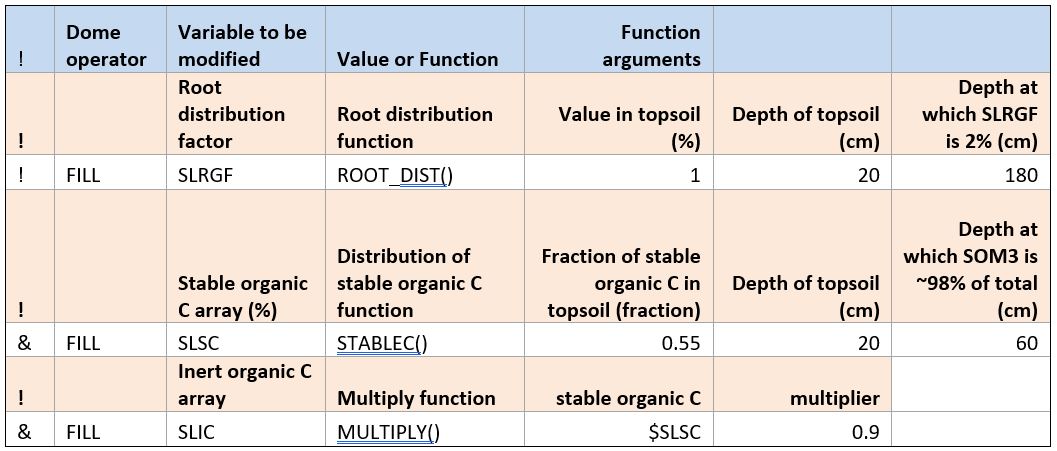
Some additional DOME functions are provided in the soil data. The ROOT_DIST() function allows the DSSAT array, soil root growth factor, to be set based on a value in the topsoil, the depth of the topsoil, and the depth at which the exponentially decaying function reaches 2% of the value in the topsoil. More information about this function is given here: ROOT_DIST - Root distribution function .

The second function used here computes stable organic C as a function of soil depth based on the STABLEC() function, described here: STABLEC - Stable C fraction distribution in soil layers.

The MULTIPLY() function simply takes one value as an argument, multiplies it by a constant, and returns the requested variable. In this case, the inert organic C array is computed as 0.9 times the stable organic C computed with the previous function.

Simulation controls

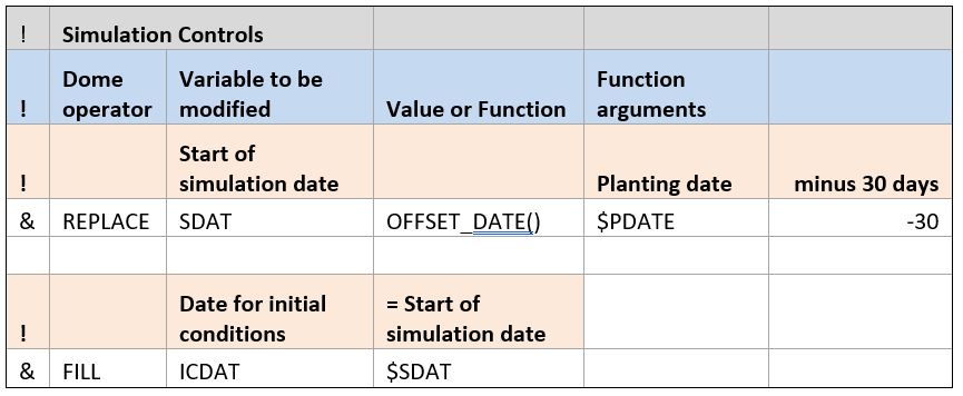
Simulation controls are model-specific and are never contained within the data collected in the field. These contain information such as when to start the simulation. In this example, the modeler chose to start the simulation 30 days prior to the planting date by using the OFFSET_DATE() function. The date associated with initial conditions was set to the start of simulation date.

Additional examples of AgMIP formatted JSON and DOME data can be found on the AgMIP Github site: https://github.com/agmip/json-translation-samples.

Connecting Experimental data with DOME data through Linkage files

If only one DOME file is specified, linkage is easy. The specified DOME is associated with each experiment and treatment (or survey element) in the dataset. But often, it is necessary to specify multiple DOMEs. For example, if the data set includes different soil types, then initial conditions may be specified for each soil type. In our Hot Serial Cereal example, no linkage file was used because the same field overlay DOME was applied to all treatments of the experiment. But if different DOMEs were applied, they would be specified in a linkage file (.lnk) as shown below. In this sample, each EXNAME is associated with one or more field overlay files. The name of the DOME is constructed from the metadata block at the top of each DOME. Multiple DOMEs can be separated by the ‘

’ (pipe) symbol, and they are applied in the order specified. Seasonal strategy DOMEs allow multiple years of execution from a single year of data and allow rules for automatic planting and irrigation to be specified for models that allow such rules. In this example, two field overlay DOMEs were specified and 3 seasonal strategy DOMEs.

DOME linkage specification:

When multiple DOME files are applied to a dataset, they should be “zipped” together and loaded into QuadUI as a zip archive file.

References

Kimball, B.A., J.W. White, G.W. Wall, M.J. Ottman 2016. Wheat Responses to a Wide Range of Temperatures: The Hot Serial Cereal Experiment. In: J. L. Hatfield, D. Fleisher, editors, Improving Modeling Tools to Assess Climate Change Effects on Crop Response, Adv. Agric. Syst. Model. 7. ASA, CSSA, and SSSA, Madison, WI. p. 33-44. doi:10.2134/advagricsystmodel7.2014.0014

Home